Compare with other neuroimaging toolbox

BEN outperforms traditional SOTA methods and advantageously adapts to datasets from various domains across multiple species, modalities, and field strengths.

Here we give one exemplar species:

1. Human (from UK-biobank)

1. Download table.

!gdown --id 1iEQo14I40feffysbZ9Ywj8amWXCD61Cc
!sh download_human_table.sh

/usr/local/lib/python3.7/dist-packages/gdown/cli.py:131: FutureWarning: Option `--id` was deprecated in version 4.3.1 and will be removed in 5.0. You don't need to pass it anymore to use a file ID.
  category=FutureWarning,
Downloading...
From: https://drive.google.com/uc?id=1iEQo14I40feffysbZ9Ywj8amWXCD61Cc
To: /content/download_human_table.sh
100% 85.0/85.0 [00:00<00:00, 108kB/s]
/usr/local/lib/python3.7/dist-packages/gdown/cli.py:131: FutureWarning: Option `--id` was deprecated in version 4.3.1 and will be removed in 5.0. You don't need to pass it anymore to use a file ID.
  category=FutureWarning,
Downloading...
From: https://drive.google.com/uc?id=1dA4NulnqgaTiDfbOxqIIi2rDkgHmhn6s
To: /content/Human_table.zip
100% 1.20M/1.20M [00:00<00:00, 87.2MB/s]
Archive:  Human_table.zip
  inflating: Fig2-violin-Human-T1.xlsx
  inflating: Fig2-vol-regress-Human-unique-T1.xlsx
  inflating: Fig2-voldiff-Human-unique-T1.xlsx

2. Violin plot (y axis: Dice score)

import seaborn as sns
import pandas as pd
import matplotlib.pyplot as plt

data = pd.read_excel(r'Fig2-violin-Human-T1.xlsx')

colors_reds = sns.color_palette('Reds')[3:]

plt.figure(figsize=(7, 5))

ax = sns.violinplot(x="Method", y="Dice", data=data[data['Method']=='AFNI'],

                    hue='Center',
                    scale='width',
                    order=['AFNI', 'FSL','Freesurfer','Sherm','Proposed'],
                    palette='Greys',
                )

ax = sns.violinplot(x="Method", y="Dice", data=data[data['Method']=='FSL'],
                    hue='Center',
                    scale='width',
                    order=['AFNI', 'FSL','Freesurfer','Sherm','Proposed'],
                    palette='Blues',

                )

ax = sns.violinplot(x="Method", y="Dice", data=data[data['Method']=='Freesurfer'],
                    hue='Center',
                    scale='width',
                    order=['AFNI', 'FSL','Freesurfer','Sherm','Proposed'],
                    palette='Greens',

                )

ax = sns.violinplot(x="Method", y="Dice", data=data[data['Method']=='BEN'],

                    hue='Center',
                    scale='width',
                    order=['AFNI', 'FSL','Freesurfer','Sherm','BEN'],
                    palette=colors_reds,

                )

plt.axvline(x=0.5, color="gray",ls="--", lw=2)
plt.axvline(x=1.5, color="gray",ls="--", lw=2)
plt.axvline(x=2.5, color="gray",ls="--", lw=2)
plt.axvline(x=3.5, color="gray",ls="--", lw=2)

plt.legend('', frameon=False)

plt.xticks(fontsize=17)
plt.yticks(fontsize=17)
plt.xlabel(xlabel='')
plt.ylabel(ylabel='')

plt.show()

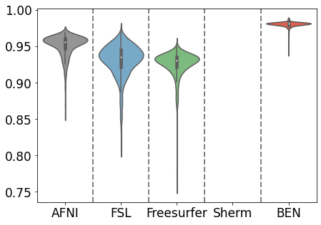
Sherm failed as it was designed for rodent.

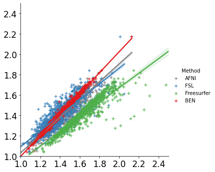
3. Regress plot

data = pd.read_excel(r'Fig2-vol-regress-Human-unique-T1.xlsx')
data['Vol']=data['Vol']/1000/1000  # (dm^3)
data['GT']=data['GT']/1000/1000

colors = sns.color_palette('Greys')[3:4]
colors.extend(sns.color_palette("Set1")[1:3])
colors.extend(sns.color_palette('Set1')[0:1])

# UKB-3T
sns.lmplot(x='Vol', y='GT', hue='Method', data=data[data['Center']=='UKB'],
           markers=['+', '+', '+', '+'],
           palette=colors,
           hue_order=['AFNI', 'FSL','Freesurfer','BEN']
          )
plt.xlim([1, 2.5])
plt.ylim([1, 2.5])

plt.xticks(fontsize=17)
plt.yticks(fontsize=17)
plt.xlabel(xlabel='')
plt.ylabel(ylabel='')

Text(32.31847222222222, 0.5, '')

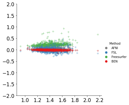
Bland–Altman analysis

data = pd.read_excel(r'Fig2-voldiff-Human-unique-T1.xlsx')
data['Diff']=data['Diff']/1000/1000  # (dm^3)
data['GT']=data['GT']/1000/1000

# UKB
sns.relplot(x='GT', y='Diff', data=data[data['Center']=='UKB'],
            hue='Method',
            hue_order=['AFNI', 'FSL','Freesurfer','BEN'],
            palette=colors,
            marker='+',
            sizes=[50,50,50,50],
            size='Method'

           )
plt.xticks(fontsize=17)
plt.yticks(fontsize=17)
plt.xlabel(xlabel='')
plt.ylabel(ylabel='')
plt.ylim([-2, 2])

(-2.0, 2.0)

Conclusion

(Details could be found in our paper)

1. As shown in Figure, despite consistent performance on human MRI scans, the AFNI, FSL, and FreeSurfer toolboxes show large intra- and inter-dataset variations on the four animal species, suggesting that these methods are not generalizable to animals.

2. Compared with other methods, BEN achieves better performance.

3. Bland–Altman analysis showing high consistency between the BEN results and expert annotations.